Learn Reinforcement Learning (2) - DQN

01 Apr 2019 • 0 Comments Tags:

[ reinforcement-learning ]

Value Function and Discount Rate
ball-find-3
Q Function
DQN

Value Function and Discount Rate

In the previous article, we introduced concepts such as discount rate, value function, as well as time to learn reinforcement learning for the first time. The two concepts are summarized again as follows.

Discount Rate: Since a future reward is less valuable than the current reward, a real value between 0.0 and 1.0 that multiplies the reward by the time step of the future time.
Value Function: A numerical representation of the value of a state.

Since the value function represents the value of a state as a number, we have looked at the value function for each state space on the Grid World and then the target can easily be found by a simple method of moving toward a grid with higher value.

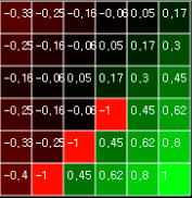Figure 1. Calculate value functions for each state in Grid World

The calculation of the value function was determined by repeated calculation until the value of each state did not change. Grid World, discussed in the last article, has fixed the location of objects and targets except the agent, so once you have calculated the value function, you could solve it easily by solving the problem.

But there are two problems here. First, even in a fixed environment, if the size of the environment is extremely large, the size of the memory for storing the value function must also increase. The environment we covered was 6x6, so we needed a storage space of 36 lengths to calculate the value function, but a 60x60 would require storage space of 3,600 lengths. Second, it is difficult to respond to a dynamic environment. If we have a large environment like 60x60, we will need several steps to calculate the value function (you need 11 steps to get the results shown in Figure 1). However, if the obstacle moves or the target moves here, we have to recalculate the value function every step.

To solve this problem, it would be better to have a fixed size input that is not affected by the size of the environment. And we should use a more efficient algorithm to solve the problem.

ball-find-3

First, let’s define the problem that corresponds to the dynamic environment. In this Grid World environment named ball-find-3, an agent and three balls are created at random locations. When the agent overlaps position with the ball, the ball disappears and agent receives a reward of +1.0, and one episode ends when all 3 balls are eliminated or 200 steps are reached. And every step gets a reward of -0.1. An agent’s action is to move one space in four adjacent directions. Here is an example of ball-find-3 where the agent picks random behavior.

let canvas = document.getElementById('editor_canvas_0');
canvas.width = 410;
canvas.height = 310;
removeClass(canvas, 'previewOutside');
addClass(canvas, 'previewOutside_410');
let ctx = canvas.getContext('2d');
let env = new Env(8, canvas);
env.maxEpisodes = 1000;
let agent = new Agent(env, Math.floor(Math.random() * 8), Math.floor(Math.random() * 8), canvas);
agent.ball_count = 3;
env.setEntity(agent, {'ball': 3});
env.draw();
agent.draw();

const post = document.getElementsByClassName('post')[0];
let button = document.createElement('button');
button.style.position = 'absolute';
button.style.top = (canvas.parentNode.offsetTop + 10).toString() + 'px';
button.width = 410 - env.grid_W * env.grid_width - 30;
button.style.left = (post.offsetLeft + post.offsetWidth - button.width - 20).toString() + 'px';
button.innerHTML = 'Step(random action)';
canvas.parentNode.appendChild(button);

let button2 = document.createElement('button');
button2.style.position = 'absolute';
button2.style.top = (canvas.parentNode.offsetTop + 35).toString() + 'px';
button2.width = 410 - env.grid_W * env.grid_width - 30;
button2.style.left = (post.offsetLeft + post.offsetWidth - button2.width - 20).toString() + 'px';
button2.innerHTML = 'Loop(random action)';
canvas.parentNode.appendChild(button2);

let is_running = false;
let rewards_array = [];

button.onclick = function() {
    if (is_running) return;
    iterate(false);
}

button2.onclick = function() {
    if (is_running) return;
    is_running = true;
    iterate(true);
}

function iterate(is_loop = true) {
    let action = Math.floor(Math.random() * 4);
    let reward, done;
    [reward, done] = agent.step(action);
    agent.reward += reward;
    agent.reward = parseFloat((agent.reward).toFixed(2));
    ctx.clearRect(0, 0, env.grid_W * env.grid_width + 10, canvas.height);

    env.steps += 1;
    env.draw();
    agent.draw();


    if (done || env.steps >= env.maxSteps) {
        rewards_array.push(Math.floor(agent.reward * 10) / 10);
        if (rewards_array.length > 1) {
            ctx.clearRect(env.grid_W * env.grid_width + 10, 0, canvas.width, canvas.height);
            env.drawRewardGraph(rewards_array.slice(rewards_array.length - 100), 255, 60);

            ctx.beginPath();
            ctx.fillStyle = 'limegreen';
            ctx.font = '14px monospace';
            let avg = rewards_array.reduce((acc, cur) => acc+cur, 0) / rewards_array.length;
            ctx.fillText(`avg. reward: ${Math.floor(avg * 10) / 10}`, env.grid_W * env.grid_width + 20, env.grid_W * env.grid_width + 60);
            ctx.closePath();
        }

        agent.x = Math.floor(Math.random() * 8);
        agent.y = Math.floor(Math.random() * 8);
        agent.reward = 0;
        agent.dir = 3;

        env.episodes += 1;
        env.steps = 0;
        env.reset();

        agent.ball_count = 3;
        while (true) {
            if (env.setEntity(agent, {'ball': 3}) !== null) {
                break;
            }
        }
    }
    if (is_loop && env.episodes < env.maxEpisodes) {
        window.requestAnimationFrame(iterate);
    }
}

window.addEventListener('resize', function() {
    button.style.top = (canvas.parentNode.offsetTop + 10).toString() + 'px';
    button.style.left = (post.offsetLeft + post.offsetWidth - button.width - 30).toString() + 'px';

    button2.style.top = (canvas.parentNode.offsetTop + 35).toString() + 'px';
    button2.style.left = (post.offsetLeft + post.offsetWidth - button2.width - 30).toString() + 'px';
});

The size of Grid World is 8x8. Theoretically, the highest point is to get all 3 balls in 3 steps and get a reward of +2.7, but this is very rare if you have a good luck, and if you usually get a small positive number or a negative number over -2.0, I think it can be said. Running an agent with a random action for 1,000 episodes gives you an average reward of about -14 to -17. Based on this, we will improve the average reward with various reinforcement learning algorithms.

Q Function

The value function we saw in the previous article was able to replace all state space with value. We were able to find the solution by finding the value function, comparing the value function to the state, and choosing the action that moves to a higher value.

In contrast, the Q function is a function that replaces a state with an action. The agents of ball-find-3 can move in four directions: up, down, left, and right. The Q function finds the value of this behavior for each state, and chooses the action with the highest Q value. This Q function is also called a policy. Q stands for Quailty and represents the quality of a particular behavior.¹

The value function is expressed as a formula \(V(s)\), and the Q function is expressed as \(Q(s,a)\). Where s is state and a is action. Unlike a value function that depends only on its state, the Q function is a value determined by its state and behavior.

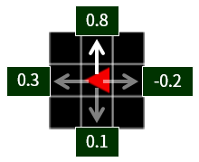Figure 2. In this position(state), the upward movement of one cell has the largest Q function value of 0.8. The agent unconditionally selects the action with high Q function value, or selects with high probability.

To update the value of a Q function, both the present value and the future value must be considered. The portion corresponding to the present value is the value of the Q function when the action(a) is taken now in the state(s).

\[Q(s,a)\]

The portion corresponding to the future value is the Q function value of the action(\(a'\)) that can be taken when the next state(\(s'\)) is reached by the action.

\[Q(s',a')\]

The actual value of a Q function can not be thought of without reward for action. If the reward is R, then the actual value of the Q function can be the sum of the reward plus the future value.

\[Q(s,a) \simeq R + Q(s',a')\]

\[Actual Value \simeq Present Value + Future Value\]

The discount rate applies to future values. Therefore, applying a discount rate to this equation multiplies \(\gamma\) by \(Q(s',a')\).

\[Q(s,a) \simeq R + \gamma Q(s',a')\]

However, the \(a'\) action that can be done in \(s'\) state is 4 moves in 4 direction in case of Grid World. Considering that you want to find the largest of the four \(Q(s',a')\), max, you can further refine the expression.

\[Q(s,a) \simeq R + \gamma maxQ(s',a')\]

Now we can see some outline. The goal is to make the value of \(Q(s,a)\) close to \(R + \gamma maxQ(s',a')\). That is, \(Q(s,a)\) is updated through reinforcement learning. The easiest way to think about it is to repeat several runs and get an average. The average of any value can be obtained by dividing the total data by the number of data. For example, when there are n-1 numbers, the average can be calculated as

\[average = \frac{1}{n-1} \sum_{i=1}^{n-1} A_{i}\]

When you want to add a new value and then try to average again, you can add all the existing values and divide by the number of data again. However, it can be transformed into the following expression.

\[\begin{align} average' & = \frac{1}{n} \left(\sum_{i=1}^{n-1} A_{i} + A_{n} \right) \\ & = \frac{1}{n} \left((n-1) \times \frac{1}{n-1} \sum_{i=1}^{n-1} A_{i} + A_{n} \right) \\ & = \frac{1}{n} ((n-1) \times average + A_{n}) \\ & = \frac{n-1}{n} \times average + \frac{A_{n}}{n} \\ & = average + \frac{1}{n} (A_{n} - average) \end{align}\]

The expression for averaging has been changed to add the difference between the new and previous averages to the previous average divided by n. At this time, \(\frac{1}{n}\) will become smaller as the number of trials increases. You can change this to a constant size number such as \(\alpha=0.1\). This \(\alpha\) is called the learning rate. By adjusting this value to increase or decrease according to the number of trials, you can lead to a better learning.

\[average' = average + \alpha(A_{n} - average)\]

Let’s introduce the expression we have summarized so far to obtain the Q function. The basic form is the same, \(\frac{1}{n}\) is \(\alpha\), average is \(Q(s,a)\), and the new value \(A_{n}\) is \(R + \gamma maxQ(s',a')\).

\[Q(s, a) = Q(s, a) + \alpha (R + \gamma max Q(s',a') - Q(s,a))\]

Now let’s try to find the Q function in a fixed environment like the value function. For the sake of smooth calculation, we will use the environment of the pit which we saw in the last article, not the ball-find-3 again. The location of the agent is fixed (x = 0, y = 0), and the location of the target and the location of the pit are fixed.

We will get a Q function for every state, all actions, as we did for the value function we looked at in the previous article. At first, initialize all to zero because there is no value at first.

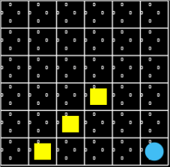Figure 3. An environment with three pits and one target in a fixed location. Each state, Q function of each action, is initialized to all 0s.

Unlike the value function, the Q function fills the table space according to the search of the agent. The agent basically chooses actions with high Q values, but it does not exploit enough to find a “moderately good” solution, which causes it to converge on it. To prevent this, we use the search method called \(\epsilon\)(epsilon)-greedy method. \(\epsilon\) is a very small number. Compares this \(\epsilon\) with a random number between 0.0 and 1.0, returns a random behavior if \(\epsilon\) is larger, otherwise it moves according to the Q function. In other words, if \(\epsilon\) is 0.3, you have 30% chance to choose random behavior.

IF randomNumber < epsilon:
    getRandomAction()
ELSE:
    getGreedyAction() // by Q

\(\epsilon\) uses a value between 0.0 and 1.0, and gradually lowers as the search progresses (cf. start value is 0.3, multiplied by 0.99 at the end of the episode, the minimum value is 0.01). This is called epsilon decay.

let canvas = document.getElementById('editor_canvas_1');
canvas.width = 410;
canvas.height = 310;
removeClass(canvas, 'previewOutside');
addClass(canvas, 'previewOutside_410');
let ctx = canvas.getContext('2d');
let env = new Env(6, canvas);
env.grid_width = 40;
env.maxEpisodes = 200;
let agent = new Agent(env, 0, 0, canvas);
agent.ball_count = 1;
env.setEntity(agent, {'ball': 1, 'box': 3}, [[5, 5], [3, 3], [2, 4], [1, 5]]);

const post = document.getElementsByClassName('post')[0];
let button = document.createElement('button');
button.style.position = 'absolute';
button.style.top = (canvas.parentNode.offsetTop + 10).toString() + 'px';
button.width = 410 - env.grid_W * env.grid_width - 30;
button.style.left = (post.offsetLeft + post.offsetWidth - button.width - 20).toString() + 'px';
button.innerHTML = 'Step';
canvas.parentNode.appendChild(button);

let button2 = document.createElement('button');
button2.style.position = 'absolute';
button2.style.top = (canvas.parentNode.offsetTop + 35).toString() + 'px';
button2.width = 410 - env.grid_W * env.grid_width - 30;
button2.style.left = (post.offsetLeft + post.offsetWidth - button2.width - 20).toString() + 'px';
button2.innerHTML = 'Loop';
canvas.parentNode.appendChild(button2);

let q_array = new Array(env.grid_W * env.grid_W * 4).fill(0);
let initial_policy_obj = {};
let idx;
for (let d = 0; d < 4; d++) {
    for (let y = 0; y < env.height; y++) {
        for (let x = 0; x < env.width; x++) {
            idx = d + x * 4 + y * 4 * env.grid_W;
            q_array[idx] = 0.0;
            initial_policy_obj[idx.toString()] = 0.0;
        }
    }
}

const gamma = 0.9;
const learning_rate = 0.1;
let epsilon = 0.3;
let epsilon_min = 0.0;
let epsilon_multiply = 0.99;

drawPolicy();
env.draw();

function drawPolicy() {
    ctx.clearRect(0, 0, env.grid_W * env.grid_width + 10, canvas.height);

    let x, y, d, m;
    for (let i = 0; i < q_array.length; i += 1) {
        x = Math.floor(i / 4) % env.grid_W;
        y = Math.floor(i / (env.grid_W * 4));
        d = i % 4;

        // not empty - not draw
        if (env.grid[y][x].length !== 0) {
            continue;
        }

        ctx.beginPath();

        if (i % 4 === 0) {
            m = Math.max(...q_array.slice(i, i+4));
        }

        if (q_array[i] === m) {
            ctx.strokeStyle = 'yellow';
            ctx.lineWidth = 2;
        }

        if (q_array[i] >= 0.0) {
            ctx.fillStyle = `rgb(0, ${Math.floor(q_array[i] * 255)}, 0)`;
        }
        else {
            ctx.fillStyle = `rgb(${Math.floor(Math.min(Math.abs(q_array[i]), 1.0) * 255)}, 0, 0)`;
        }


        ctx.moveTo((x + 0.5) * env.grid_width, (y + 0.5) * env.grid_width);
        ctx.lineTo((x + dirs_tri[d][0][0]) * env.grid_width, (y + dirs_tri[d][0][1]) * env.grid_width);
        ctx.lineTo((x + dirs_tri[d][1][0]) * env.grid_width, (y + dirs_tri[d][1][1]) * env.grid_width);
        ctx.lineTo((x + 0.5) * env.grid_width, (y + 0.5) * env.grid_width);
        ctx.fill();

        if (q_array[i] === m) {
            ctx.stroke();
        }

        //ctx.fillRect(x * env.grid_width, y * env.grid_width, env.grid_width, env.grid_width);
        ctx.closePath();
    }

    ctx.beginPath();
    ctx.fillStyle = 'white';
    ctx.font = '7px monospace';
    for (let i = 0; i < q_array.length; i += 1) {
        x = Math.floor(i / 4) % env.grid_W;
        y = Math.floor(i / (env.grid_W * 4));
        d = i % 4;

        // not empty - not draw
        if (env.grid[y][x].length !== 0) {
            continue;
        }

        ctx.fillText(q_array[i], (x+0.5+dirs[d][0] * 0.3) * env.grid_width - 8, (y+0.5+dirs[d][1] * 0.3) * env.grid_width);
    }
    ctx.closePath();

    env.drawOutline();
}

button.onclick = function() {
    iterate(false);
}

button2.onclick = function() {
    iterate(true);
}

let is_running = false;
let rewards_array = [];

function iterate(is_loop = true) {
    let q_s = [];
    let x, y, state_idx;
    state_idx = (agent.x + agent.y * env.grid_W) * 4;
    q_s = q_array.slice(state_idx, state_idx + 4);

    // find max q
    const m = Math.max(...q_s);
    q_s = q_s.map((c,i) => c == m ? i : -1).filter(c => c >= 0);
    let action;

    // epsilon-greedy
    if (Math.random() < epsilon) {
        action = Math.floor(Math.random() * 4);
    }
    else {
        action = q_s[Math.floor(Math.random() * q_s.length)];
    }

    let reward, done;
    [reward, done] = agent.step(action);
    let next_state_idx = (agent.x + agent.y * env.grid_W) * 4;

    // update q
    q_array[state_idx + action] += learning_rate * (reward + gamma * Math.max(...q_array.slice(next_state_idx, next_state_idx + 4)) - q_array[state_idx + action]);

    q_array[state_idx + action] = Math.floor(q_array[state_idx + action] * 100) / 100;

    agent.reward += reward;
    agent.reward = parseFloat((agent.reward).toFixed(2));
    ctx.clearRect(0, 0, env.grid_W * env.grid_width + 10, canvas.height);

    env.steps += 1;
    drawPolicy();
    env.draw();
    agent.draw();


    if (done || env.steps >= env.maxSteps) {
        rewards_array.push(Math.floor(agent.reward * 10) / 10);
        if (rewards_array.length > 1) {
            ctx.clearRect(env.grid_W * env.grid_width + 10, 0, canvas.width, canvas.height);
            env.drawRewardGraph(rewards_array, 255, 80);

            ctx.beginPath();
            ctx.fillStyle = 'white';
            ctx.font = '14px monospace';
            ctx.fillText(`epsilon: ${epsilon}`, env.grid_W * env.grid_width + 20, env.grid_W * env.grid_width + 40);
            ctx.closePath();
        }

        agent.x = 0;
        agent.y = 0;
        agent.reward = 0;
        agent.dir = 3;
        agent.ball_count = 1;

        env.episodes += 1;
        env.steps = 0;
        env.reset();

        // epsilon_decay
        if (epsilon > epsilon_min) {
            epsilon = epsilon * epsilon_multiply;
            epsilon = Math.floor(epsilon * 10000) / 10000;
        }

        while (true) {
            if (env.setEntity(agent, {'ball': 1, 'box': 3}, [[5, 5], [3, 3], [2, 4], [1, 5]]) !== null) {
                break;
            }
        }
    }
    if (is_loop && env.episodes < env.maxEpisodes) {
        window.requestAnimationFrame(iterate);
    }
}

window.addEventListener('resize', function() {
    button.style.top = (canvas.parentNode.offsetTop + 10).toString() + 'px';
    button.style.left = (post.offsetLeft + post.offsetWidth - button.width - 30).toString() + 'px';

    button2.style.top = (canvas.parentNode.offsetTop + 35).toString() + 'px';
    button2.style.left = (post.offsetLeft + post.offsetWidth - button2.width - 30).toString() + 'px';
});

// because of mathjax.. reset position
var el = document;
var event = document.createEvent('HTMLEvents');
event.initEvent('resize', true, false);
setTimeout(function() {el.dispatchEvent(event);}, 1000);

Pressing the Step button moves the agent one step, pressing the Loop button automatically continues until the agent reaches maxEpisode.

The value of the Q function is updated as time goes by. The Q value that makes the action to reach the target in a state close to the target changes to green (positive number), and the value next to the pit changes to red (negative number). The yellow triangle represents the value of the Q function corresponding to max in each state. After approximately 100 episodes, the epsilon value is lowered and the optimal solution of the Q function is found.

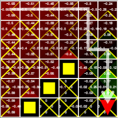Figure 4. The agent can reach its goal by following the yellow triangle, which means the max Q value of each state.

In the fixed state, the optimal solution can be found by filling the Q table of the value of the Q function, that is, the \(state(s) \time behavior(a)\) size. In the Grid World above, \(36 \times 4 = 144\). But how do we cope if the size of the environment we considered is very large?

First, we need a basic premise that the size of the input should be constant no matter how large the environment is. Otherwise, considering all the states of the environment, the memory needed to calculate the behavior will increase proportionally to the size of the environment.

Even in the real environment where the robot learns, the range of the sensor that detects the surroundings is limited, and the agent’s field of view can be arbitrarily limited so that only the information in the field of view can be received and judged.

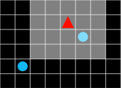Figure 5. The field of view is bright.

When this occurs, each state becomes the current state of all objects in the field of view. Not only which cell the agent is located in, but also the state value of what landscape is visible in the agent’s field of view. The state value should be changed even if it changes slightly in the landscape. In other words, the size of the state memory can grow exponentially, not proportional to the size of the field of view.

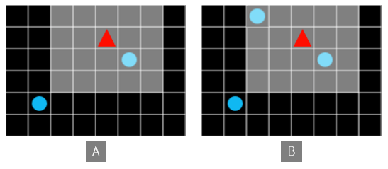Figure 6. A and B are treated differently.

Therefore, you can not save a Q function as a table, as you did above. One way to think about this is to use a neural network that effectively stores large amounts of data and turns that data into efficient function outputs. DQN came out at this point.

DQN

In Deepmind’s historical paper, “Playing Atari with Deep Reinforcement Learning”, they announced an agent that successfully played classic games of the Atari 2600 by combining Deep Neural Network with Q-Learning using Q functions. Especially in some games, DQN has become more talked about because it gets scores that surpass human play.

Figure 7. The agent learning with DQN is playing Atari-breakout. The agent learns for himself and finds the best solution for sending the ball to the back of the block line. Source Link

This algorithm receives a game screen corresponding to 4 consecutive frames as an input of the Convolution network, and then learns a Q function that maximizes reward through a Q-learning process. Just as a person plays the game, the agent will play the game with the appropriate keystrokes at the given screen.

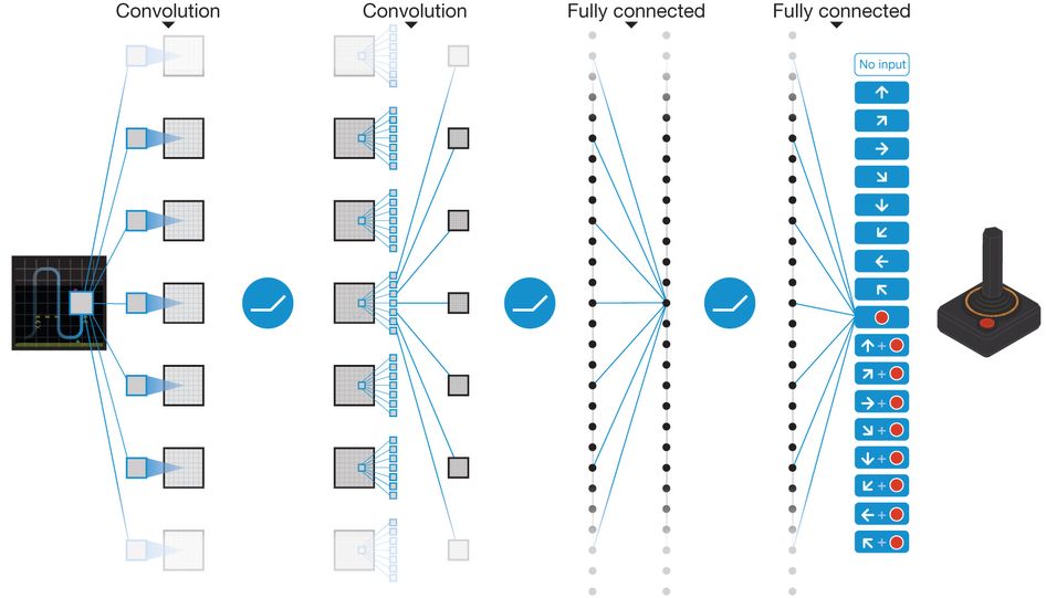Figure 8. The schematic network structure of DQN. Source Link

In the above fixed environment Q-Learning, if the state is replaced with the behavior through the Q table, the DQN replaces the state with the behavior through the Q network. Deep learning networks can overcome the limitations of conventional table-based memory and learn efficient function output for large amounts of data.

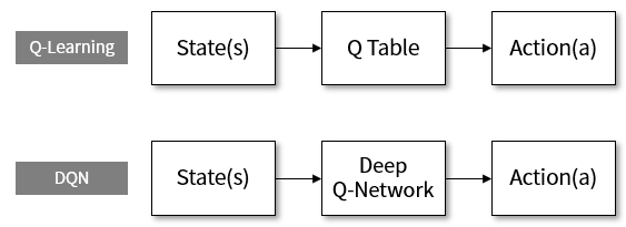Figure 9. DQN stands for Deep Q-Network.

In addition to the basic idea of replacing the table of Q function with the network, the DQN thesis includes ideas such as experience replay and target network to improve performance. It would seem to be beyond the scope of this article to elaborate on these, so if you are interested, this article will be helpful.

Let’s implement DQN in Grid World environment. We will use tensorflow-js as the Deep Learning library. tensorflow-js is a javascript version of tensorflow, the most widely used deep-running framework in the world today. It is compatible with tensorflow on model, and supports concise API usage that is affected by keras.

The network structure we use is simpler than Figure 8. After receiving the input corresponding to the view of the agent, it compresses the image information using the convolution layer and captures the feature. Then connect the dense layer and finally connect the dense layer with four nodes equal to the size of the action, and use the output of the network as the agent’s action.

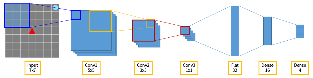Figure 10. The schematic network structure of Grid World-DQN.

let global_step = 0;
let canvas = document.getElementById('editor_canvas_2');
canvas.width = 410;
canvas.height = 310;
removeClass(canvas, 'previewOutside');
addClass(canvas, 'previewOutside_410');
let ctx = canvas.getContext('2d');
let env = new Env(8, canvas);
env.maxEpisodes = 2000;
let agent = new DQNAgent(env, Math.floor(Math.random() * 8), Math.floor(Math.random() * 8), canvas);
agent.ball_count = 3;
agent.vision = true;
env.setEntity(agent, {'ball': 3});
env.draw();
agent.draw();

const post = document.getElementsByClassName('post')[0];
let button = document.createElement('button');
button.style.position = 'absolute';
button.style.top = (canvas.parentNode.offsetTop + 10).toString() + 'px';
button.width = 410 - env.grid_W * env.grid_width - 30;
button.style.left = (post.offsetLeft + post.offsetWidth - button.width - 20).toString() + 'px';
button.innerHTML = 'Learn(DQN)';
canvas.parentNode.appendChild(button);

let button2 = document.createElement('button');
button2.style.position = 'absolute';
button2.style.top = (canvas.parentNode.offsetTop + 35).toString() + 'px';
button2.width = 410 - env.grid_W * env.grid_width - 30;
button2.style.left = (post.offsetLeft + post.offsetWidth - button2.width - 20).toString() + 'px';
button2.innerHTML = 'Run(DQN)';
button2.disabled = true;
canvas.parentNode.appendChild(button2);

let is_running = false;
let rewards_array = [];

let epsilon = 0.3;
let epsilon_min = 0.0;
let epsilon_multiply = 0.99;

button.onclick = function() {
    if (is_running) return;
    is_running = true;
    iterate(true);
}

button2.onclick = function() {
    if (is_running) return;
    is_running = true;
    env.maxEpisodes += 1;

    agent.x = Math.floor(Math.random() * 8);
    agent.y = Math.floor(Math.random() * 8);
    agent.reward = 0;
    agent.dir = 3;

    // env.episodes += 1;
    env.steps = 0;
    env.reset();

    agent.ball_count = 3;
    while (true) {
        if (env.setEntity(agent, {'ball': 3}) !== null) {
            break;
        }
    }

    run();
}

function getAction(agent, input) {
    if (Math.random() < epsilon) {
        return Math.floor(Math.random() * 4);
    }
    return tf.tidy(() => {
        let inputTensor = tf.tensor4d(input, [1, 7, 7, 1]);
        //const logits = agent.model.predict(inputs.reshape([1, 7, 7, 1]));
        const logits = agent.model.predict(inputTensor);
        const softmax = logits.softmax();
        const actions = tf.multinomial(softmax, 1, null, true);
        return actions.dataSync()[0];
    });
}

function getVision(agent) {
    let top, left;
    left = agent.x - agent.visionForward;
    top = agent.y - agent.visionForward;
    let s = [];

    for (let y = top; y < top + agent.visionForward * 2 + 1; y += 1) {
        for (let x = left; x < left + agent.visionForward * 2 + 1; x += 1) {
            if (x >= 0 && x < env.width &&
                y >= 0 && y < env.height) {
                if (env.grid[y][x].length > 0) {
                    s.push(object_to_idx[env.grid[y][x][0].type]);
                }
                else {
                    s.push(object_to_idx['empty']);
                }
            }
            else {
                s.push(object_to_idx['unseen']);
            }
        }
    }

    return s;
}

function run(is_loop = true) {
    const state = getVision(agent);
    const action = getAction(agent, state);
    let reward, done;
    [reward, done] = agent.step(action);
    agent.reward += reward;
    agent.reward = parseFloat((agent.reward).toFixed(2));

    ctx.clearRect(0, 0, env.grid_W * env.grid_width + 10, canvas.height);

    env.steps += 1;
    env.draw();
    agent.draw();

    if (done || env.steps >= env.maxSteps) {
        rewards_array.push(Math.floor(agent.reward * 10) / 10);
        if (rewards_array.length > 1) {
            ctx.clearRect(env.grid_W * env.grid_width + 10, 0, canvas.width, canvas.height);
            env.drawRewardGraph(rewards_array.slice(rewards_array.length - 100), 255, 60);

            ctx.beginPath();
            ctx.fillStyle = 'limegreen';
            ctx.font = '14px monospace';
            let avg = rewards_array.reduce((acc, cur) => acc+cur, 0) / rewards_array.length;
            ctx.fillText(`avg. reward: ${Math.floor(avg * 10) / 10}`, env.grid_W * env.grid_width + 20, env.grid_W * env.grid_width + 60);
            ctx.closePath();
        }
    }
    if (is_loop && env.episodes < env.maxEpisodes) {
        window.requestAnimationFrame(iterate);
    }
}

async function iterate(is_loop = true) {
    const state = getVision(agent);
    const action = getAction(agent, state);
    let reward, done;
    [reward, done] = agent.step(action);
    agent.reward += reward;
    agent.reward = parseFloat((agent.reward).toFixed(2));
    const next_state = getVision(agent);
    agent.append_sample(state, action, reward, next_state, done);

    ctx.clearRect(0, 0, env.grid_W * env.grid_width + 10, canvas.height);

    env.steps += 1;
    env.draw();
    agent.draw();

    global_step += 1;
    if (global_step % agent.learn_step === 0) {
        // if (agent.memory.getLength() >= agent.train_start) {
        if (agent.memory.length >= agent.train_start) {
            await agent.train_model();
        }
    }

    if (done || env.steps >= env.maxSteps) {
        rewards_array.push(Math.floor(agent.reward * 10) / 10);
        if (rewards_array.length > 1) {
            ctx.clearRect(env.grid_W * env.grid_width + 10, 0, canvas.width, canvas.height);
            env.drawRewardGraph(rewards_array.slice(rewards_array.length - 100), 255, 60);

            ctx.beginPath();
            ctx.fillStyle = 'white';
            ctx.font = '14px monospace';
            ctx.fillText(`epsilon: ${epsilon}`, env.grid_W * env.grid_width + 20, env.grid_W * env.grid_width + 40);
            ctx.closePath();

            ctx.beginPath();
            ctx.fillStyle = 'limegreen';
            ctx.font = '14px monospace';
            let avg = rewards_array.reduce((acc, cur) => acc+cur, 0) / rewards_array.length;
            ctx.fillText(`avg. reward: ${Math.floor(avg * 10) / 10}`, env.grid_W * env.grid_width + 20, env.grid_W * env.grid_width + 60);
            ctx.closePath();
        }

        agent.x = Math.floor(Math.random() * 8);
        agent.y = Math.floor(Math.random() * 8);
        agent.reward = 0;
        agent.dir = 3;

        env.episodes += 1;
        env.steps = 0;
        env.reset();

        // epsilon_decay
        if (epsilon > epsilon_min) {
            epsilon = epsilon * epsilon_multiply;
            epsilon = Math.floor(epsilon * 10000) / 10000;
        }

        await agent.update_target_model();

        agent.ball_count = 3;
        while (true) {
            if (env.setEntity(agent, {'ball': 3}) !== null) {
                break;
            }
        }
    }
    if (is_loop && env.episodes < env.maxEpisodes) {
        window.requestAnimationFrame(iterate);
    }
    else {
        button.disabled = true;
        button2.disabled = false;
        is_running = false;
    }
}

window.addEventListener('resize', function() {
    button.style.top = (canvas.parentNode.offsetTop + 10).toString() + 'px';
    button.style.left = (post.offsetLeft + post.offsetWidth - button.width - 30).toString() + 'px';

    button2.style.top = (canvas.parentNode.offsetTop + 35).toString() + 'px';
    button2.style.left = (post.offsetLeft + post.offsetWidth - button2.width - 30).toString() + 'px';
});

When you press the Learn (DQN) button, the agent starts learning. Since the experience replay is applied, the agent stores all the information it experiences in memory in the form of (state, action, reward, next_state, done), and starts learning from the time when a certain number of information (train_start=1000) accumulates. Each time 10 steps(learn_step=10) passes, we use 64 samples(batch_size=64) extracted from memory.

When I study up to 2000 episodes, the average reward is -11~-12. This is an improvement over the -14~-17 of random action agents. We can try to adjust the hyper parameters of the deep running - train_start, learn_step, batch_size, etc. and get a better average reward. We can also modify the network structure or apply a more advanced algorithm (A2C, PPO, etc.) to increase the average reward.

With a limited field of view, we have found that DQN agents can outperform random action agents in relatively difficult problems where agents and balls are created at random locations. However, it seems that the ratio of going straight to the ball and going to the other side is similar. Next time I will explain how to make this agent more efficient, and more efficient algorithms to solve the more difficult problems. Thank you for reading the long article.

DEMYSTIFYING DEEP REINFORCEMENT LEARNING ↩

greentec's blog game designer, scripter, researcher

Learn Reinforcement Learning (2) - DQN

Value Function and Discount Rate

ball-find-3

Q Function

DQN

Related Posts

CoG 2019 attendance review 29 Aug 2019

Learn Reinforcement Learning (5) - Solving problems with a door and a key 09 Jun 2019

Learn Reinforcement Learning (4) - Actor-Critic, A2C, A3C 07 May 2019