Learn Reinforcement Learning (3) - DQN improvement and Deep SARSA

16 Apr 2019 • 0 Comments

• DQN improvement
  • Hyperparameter adjustment
  • weight initialization
  • soft update (target network)
  • Double DQN
  • Dueling DQN
• Deep SARSA

In the previous article, we learned the DQN in Grid World that was developed by Deepmind and used to play Atari games. The average reward of the random action agent was obtained from -14 to -17, whereas the average reward of the DQN agent was obtained from -11 to -12.

However, if you move the learned agent by pressing the Run button, you can not show satisfactory movements such as wandering in front of the goal. Today, after DQN was first announced in 2013, we will try to increase the average reward of the ball-find-3 problem in Grid World by applying various methods to improve performance. Next, we will look at a more efficient algorithm for solving this problem.

 

DQN improvement

Hyperparameter adjustment

The easiest way to think about is to adjust the hyper parameters. Hyper parameters include the learning rate, batch size, etc. that affect the learning of the deep learning network. Also specific to DQN is the total size of the memory to store the experience, the memory size at which to start learning, and the discount rate, \(\gamma\).

Figure 1. Hyperparameter adjustments can be likened to adjusting the number of switches to achieve the desired results. Source Link

We can adjust the learn_step. The previous article’s DQN agent was set to learn_step=10, so agent learned every 10 steps. How about reducing this step? Of course the agent will learn more often. Does learning average increase the average reward? If learn_step=1, the agent will learn 10 times faster by learning every step.

weight initialization

Deep learning networks consist of a number of float value weights and bias. These values determine the output of the deep learning, but before the learning begins, these values are undefined and need to be initialized. The usual way to do this is to initialize to a random number, but we can use Glorot Initialization to create an initial value for the weight that yields a more stable result. This method is also called Xavier Initialization because it was proposed by a person named Xavier Glorot.¹

soft update (target network)

As I mentioned in the last article, DQN has an idea of target network. Q-Learning updates the Q-value as follows.

\[Q(s, a) = Q(s, a) + \alpha (R + \gamma max Q(s', a') - Q(s, a))\]

Where \(\alpha\) is the learning rate. In the update equation, \(Q(s, a)\) is updated by multiplying \(R + \gamma max Q(s', a') - Q(s, a)\) by \(\alpha\). If \(\alpha=0\), \(Q(s, a)\) will not change, and if \(\alpha=1\), \(Q(s, a)\) will be\(R + \gamma max Q(s',a')\). Since \(\alpha\) is usually between 0.0 and 1.0, you can think of this update expression as:

\[Q(s, a) = Q(s, a) + \alpha (\underbrace{R + \gamma max Q(s', a')}_{target} - Q(s, a))\] \[Q(s, a) \rightarrow R + \gamma max Q(s', a')\]

That is, when learning continues, \(Q(s, a)\) approaches \(R + \gamma max Q(s', a')\). If we denote the weight and bias of Q-network as \(\theta\), we can use the above equation as follows.

\[Q(s, a;\theta) \rightarrow R + \gamma max Q(s', a';\theta)\]

The problem with this equation is that the current value and the goal use the same network weight. The weight of the Q-network changes with each learning. However, since the goal also changes, it may be difficult to converge to a certain value. Therefore, a separate network with the same structure as the Q-network named target network is created and marked with the symbol \(\theta^{-}\).

\[Q(s, a;\theta) \rightarrow R + \gamma max Q(s', a';\theta^{-})\]

The target network maintains a fixed value during the learning process of the original Q-network², and then periodically resets it to the original Q-network value. This can be effective learning because the Q-network can be approached with a fixed target network.

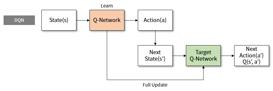Figure 2. Structure of learning using target network in DQN

A soft update means that we do not update this target network at once, but frequently and very little. The value of \(\tau\) is used. In Deepmind’s paper³, which proposed an algorithm called DPG, they used \(\tau=0.001\). The target network is updated as follows.

\[\theta^{-} = \theta \times \tau + \theta^{-} \times (1 - \tau)\]

The target network will move slightly to the value of Q-network. Since the value of \(\tau\) is small, the update should be frequent so that the effect will be noticeable. I modified the code to soft update every time agent learned.

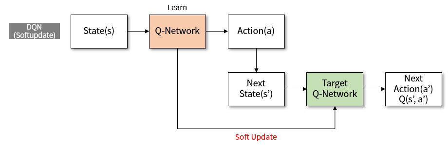Figure 3. The structure of learning to soft update target network in DQN

Let’s try the above three enhancements, the agent that applied learn_step adjustment + soft update (target network) + weight initialization (glorot initialization).

By clicking on the Learn (DQN) button, you can get an average reward of -9 to -10 by running the DQN algorithm with several changes to the 2000 episode. This is slightly better than -11 to -12 of pure DQN.

 

 

Double DQN

David Silver of Deepmind cited three major improvements since Nature DQN in his lecture entitled “Deep Reinforcement Learning”.⁴ Three things are Double DQN, Prioritized replay, and Dueling DQN. Let’s look at the double DQN and the Dueling DQN that have changes in the direct calculation.

Double DQN was an algorithm that used two Q-networks to improve the Q-Learning problem in 2010, before the original DQN. In the “Double Q-Learning” paper by Hado van Hasselt, he pointed out that Q-learning tends to be difficult because of the tendency of overestimating Q-values.

\[Q(s, a) = Q(s, a) + \alpha (R + \gamma max Q(s', a') - Q(s, a))\]

In the original Q-learning equation, when \(max Q(s', a')\) is extracted, this value is obtained by selecting \(a'\) having the highest Q value in the Q-network when the state \(s'\) is given, by multiplying the Q value by \(\gamma\), so that will create a target value that \(Q(s, a)\) should be close. However, the problem is that you use the same Q-network in the 1. Select, 2. Import Q values. Because the max operation is used, the selected Q value is usually a large value, and the Q value will go in the increasing direction because it gets its value. However, if the Q value becomes larger than necessary, the performance of the Q-network will be greatly degraded.

To prevent this, Hado van Hasselt’s first approach is to use two Q-networks.

\[Q_{A}(s, a) = Q_{A}(s, a) + \alpha (R + \gamma Q_{B}(s', argmaxQ_{A}(s',a')) - Q_{A}(s, a))\] \[Q_{B}(s, a) = Q_{B}(s, a) + \alpha (R + \gamma Q_{A}(s', argmaxQ_{B}(s',a')) - Q_{B}(s, a))\]

The two expressions are the same if A and B are changed. Based on the above equation, the \(argmaxQ_{A}(s',a')\) part is the part of the \(Q_{A}\) network that selects the behavior. And the outer \(Q_{B}(s', argmaxQ_{A}(s',a'))\) gets the Q value from the \(Q_{B}\) network. The use of two Q-networks together is key to Double DQN’s ability to prevent unnecessarily large Q values.

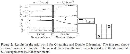Figure 4. In the “Double Q-Learning” example, the Grid world was a small 3x3. In the lower right, S is the starting point and G is the target point.

However, as we have seen above, DQN already had the idea of ​​a target network. Hado van Hasselt, who wrote this paper, went to Deepmind and published “Deep Reinforcement Learning with Double Q-learning” with David Silver, a paper that applied Double Q-Learning to DQN in 2016.

\[Q(s, a;\theta) \rightarrow R + \gamma max Q(s', a';\theta^{-})\]

The above equation changes as follows.

\[Q(s, a;\theta) \rightarrow R + \gamma max Q(s', argmaxQ(s',a';\theta);\theta^{-})\]

Use the existing Q-network to select the action, and get the Q value from the target network with the selected behavior. There are so many formulas that I think it might be hard to see. As shown above, the learning structure diagram is as follows.

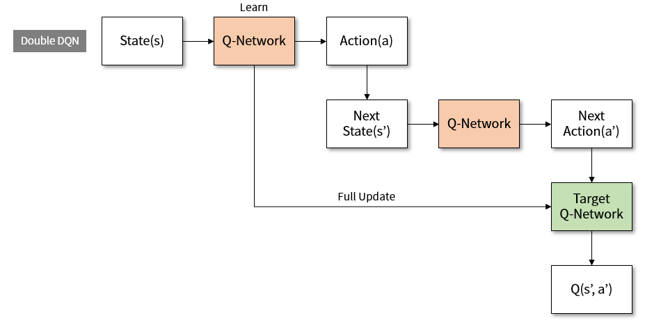Figure 5. Learning structure of Double DQN

Let’s look at the results of applying the Double DQN with the interactive example.

Double DQN and the Dueling DQN described later also have soft update, learn step 10->1, and glorot initialization. Since reinforcement learning can vary depending on execution, I have shown graphs of performance of Random, DQN, DQN-softupdate and Double DQN.

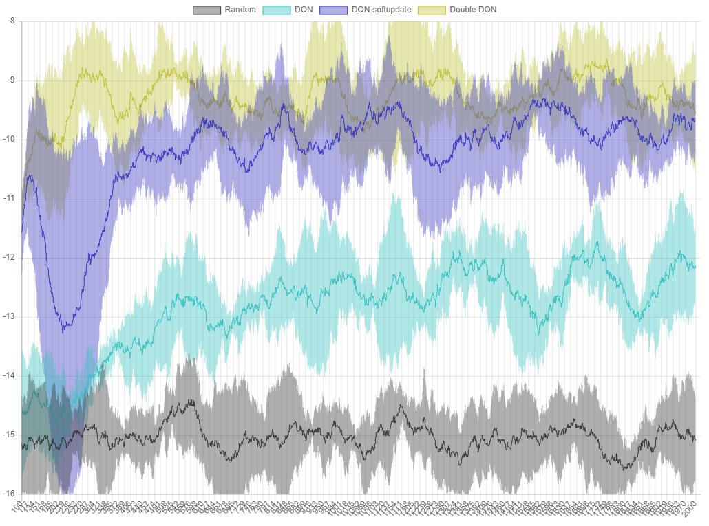Figure 6. The performance graph of each algorithm in ball-find-3. The X axis is the episode, and the Y axis is the average of the rewards from the last 100 trials.

Each algorithm has five runs, the average value is the line, and the maximum and minimum values are in the area. You can see that the version with Double DQN has better performance than DQN-softupdate.

Dueling DQN

Dueling DQN is an idea of ​​dividing the network result by V and A, then reassembling it and then getting the Q value. V is equivalent to the value function we saw in the first article of this series, and A is the value Advantage. Since A is calculated value for each action, it is easy to think that it is similar to Q value. The important point here is that V can be calculated. Calculate V for each state and add it to Q as shown below.

\[Q(s, a) = V(s) + A(s, a) - \frac{1}{|A|}\sum_{a} A(s, a)\]

Since the V values are added together when the Q value is obtained, the Q value of the state having a high V value will increase as a result, and in the opposite case, the Q value will be lowered. Therefore, the agent moves to a state with a high Q value (high V), avoiding the action of giving a low Q value (low V). This idea of separating information about values and behaviors is similarly applied to the Actor-Critic algorithm, which we will introduce next time.

Unlike the above Double DQN, Dueling DQN changes network structure. At the end, the output layer that selects the action is the same, but in the middle, V and A are calculated separately, and finally reassembled and the Q value is calculated to select the action.

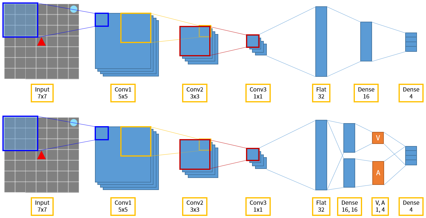Figure 7. The above is the DQN network structure in Grid World, and below is Dueling DQN.

The performance of Dueling DQN is also better than the existing soft update version. Double DQN and Dueling DQN are also called DDDQN(Dueling Double Deep Q-Network).

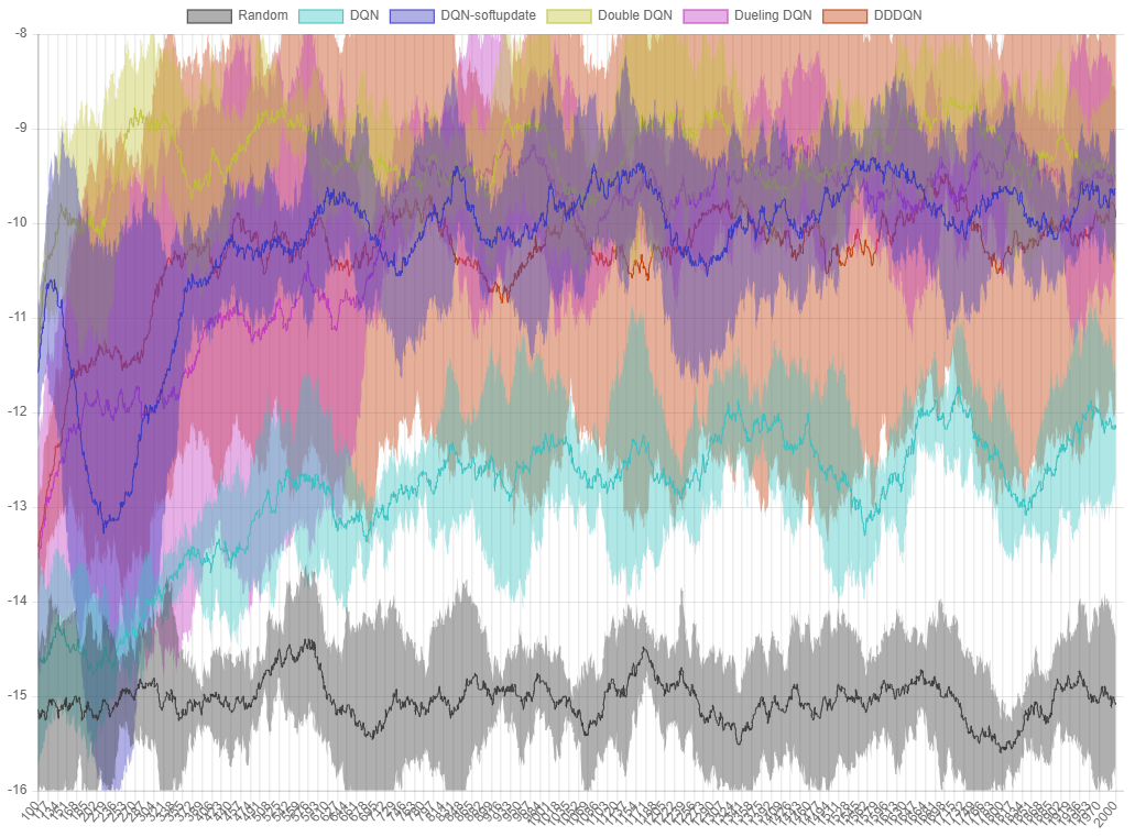Figure 8. The performance graph of each algorithm in ball-find-3. The X axis is the episode, and the Y axis is the average of the rewards from the last 100 trials.

Dueling DQN shows better performance than DQN and has similar performance to soft update version. DDDQN, which combines Dueling and Double, did not record very good performance in this problem, but it seems to be able to improve the results through parameter tuning and so on.

 

Deep SARSA

Some problems may be more effective with simple algorithms than with complex algorithms. In this Grid World, for the ball-find-3 problem, the Deep SARSA algorithm performed better than the DQN. SARSA is a combination of state(s), action(a), reward(r), next state(s’), and next action(a’) that we have seen above.

Comparing Q-learning with SARSA, it can be said that SARS uses only state(s), action(a), reward(r), and next state(s’). So the difference between Q-learning and SARSA is whether the next action(a’) is necessary for learning.

\[Q-learning : Q(s, a) = Q(s, a) + \alpha (R + \gamma max Q(s', a') - Q(s, a))\] \[SARSA : Q(s, a) = Q(s, a) + \alpha (R + \gamma Q(s', a') - Q(s, a))\]

SARSA expressions include \(Q(s', a')\) instead of missing the max operator. If Q-learning is a greedy way of finding the max-Q value of the next step, then SARSA is a stochastic way of using the value of the action the agent took in the next step directly. Q-learning is an off-policy algorithm that must be performed after episode execution because max value must be obtained, but SARSA also has an attribute called on-policy algorithm that can be learned at any time during episode execution.

Deep SARSA is a deep learning neural network that uses Q-network to obtain Q value like DQN. Let’s look at an interactive example of how well Deep SARSA performs in this problem.

The DeepSARSA agent gets an average reward of about -8 to -10. If you press the RUN (DeepSARSA) button after the learning ends, you can see that agent movement is more efficient than DQN.

So far, we have looked at several ways to improve DQN and DeepSARSA, which is similar to DQN but on-policy. Next time, we will look at Actor-Critic, which has a concept similar to Dueling DQN. In addition, I attached the motion of the agent who trained the ball-find-3 problem with the Actor-Critic algorithm for 2,000 episodes. Let’s analyze this algorithm next time.

Figure 9. Actor-Critic agent. In ball-find-3, the average reward is -2.5~-1.5.

And I have summarized the performance of the algorithms we have seen so far. Because it is an interactive graph, you can turn on / off the top item and compare only the items you want to see.

It seems that you could be burdened by the fact that the formula was much larger than the previous article. It is not easy, but I will try to solve it as easily as possible next time. Thank you for reading the long article.